
Like RColorBrewer and MetBrewer, PortinariColors groups its palettes by the kind of data they suit.
portinari.palettes()[, c("palette", "category", "n_colors", "cvd_n")]## palette category n_colors cvd_n
## 1 cafe qualitative 6 6
## 2 paz qualitative 8 4
## 3 retirantes diverging 8 8
## 4 inah diverging 5 4
## 5 sofia diverging 5 3
## 6 terra_roxa diverging 9 9
## 7 guerra diverging 9 9
## 8 guerra_azul sequential 6 6
## 9 roxa_terra sequential 8 8
## 10 paz_ouro sequential 4 4Qualitative: unordered groups
Distinct hues with no implied order. Asking for n colors
returns the n most distinct ones.
show_portinari(category = "qualitative")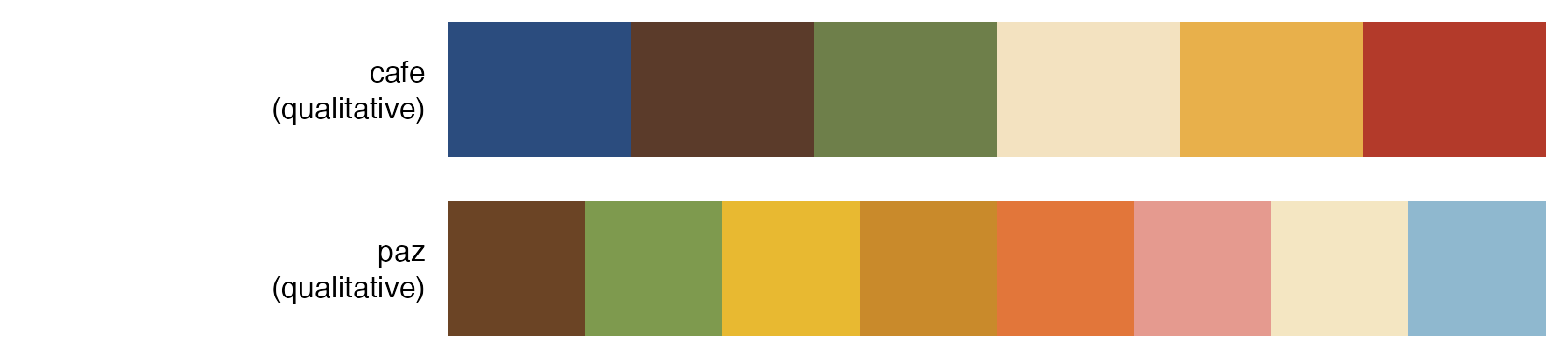
ggplot(mpg, aes(displ, hwy, colour = drv)) +
  geom_point(size = 2.5, alpha = 0.8) +
  scale_color_portinari("cafe", name = "Drive")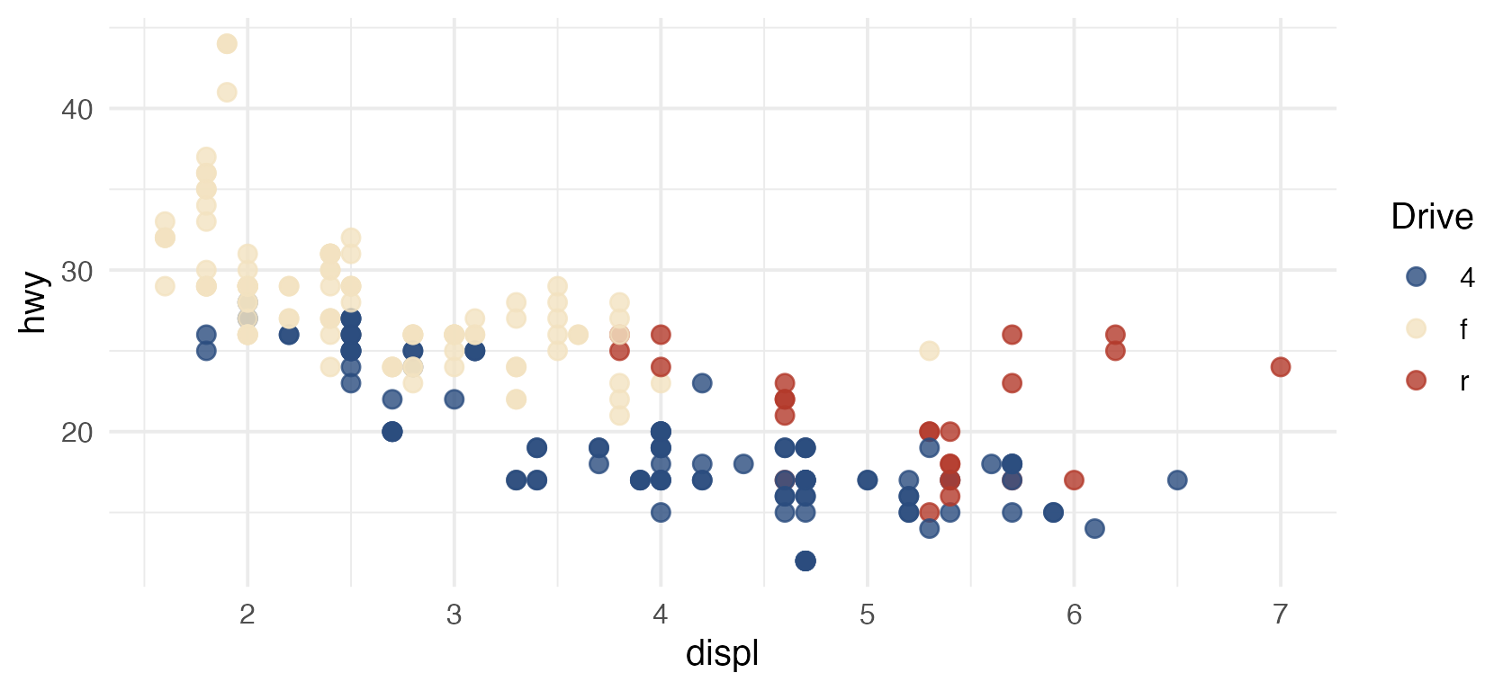
Sequential: ordered values
Colors run from dark to light. Discrete subsets keep both ends and space the rest evenly.
show_portinari(category = "sequential")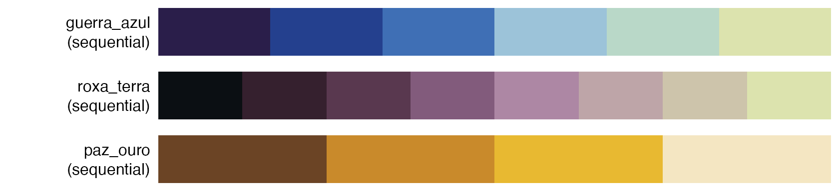
ggplot(faithfuld, aes(waiting, eruptions, fill = density)) +
  geom_raster() +
  scale_fill_portinari("guerra_azul", type = "continuous", direction = -1) +
  coord_cartesian(expand = FALSE)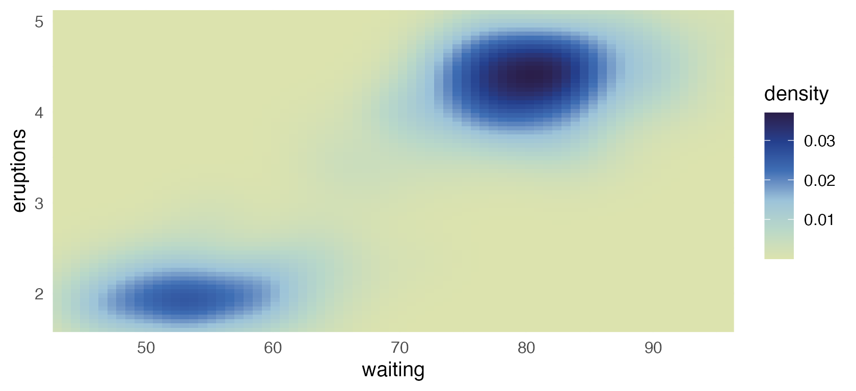
roxa_terra runs from the soil black of Coffee
Agricultural Worker through its plums to the pale citrine of
Guerra, the lightest color of guerra_azul, so even
its lightest values stay visible on a white page. Here it maps the
elevation of Maungawhau volcano.
volcano_long <- data.frame(
  x = rep(seq_len(nrow(volcano)), ncol(volcano)),
  y = rep(seq_len(ncol(volcano)), each = nrow(volcano)),
  height = as.vector(volcano)
)
ggplot(volcano_long, aes(x, y, fill = height)) +
  geom_raster() +
  scale_fill_portinari("roxa_terra", type = "continuous", direction = -1,
                       name = "Height (m)") +
  coord_equal(expand = FALSE) +
  labs(x = NULL, y = NULL) +
  theme(axis.text = element_blank())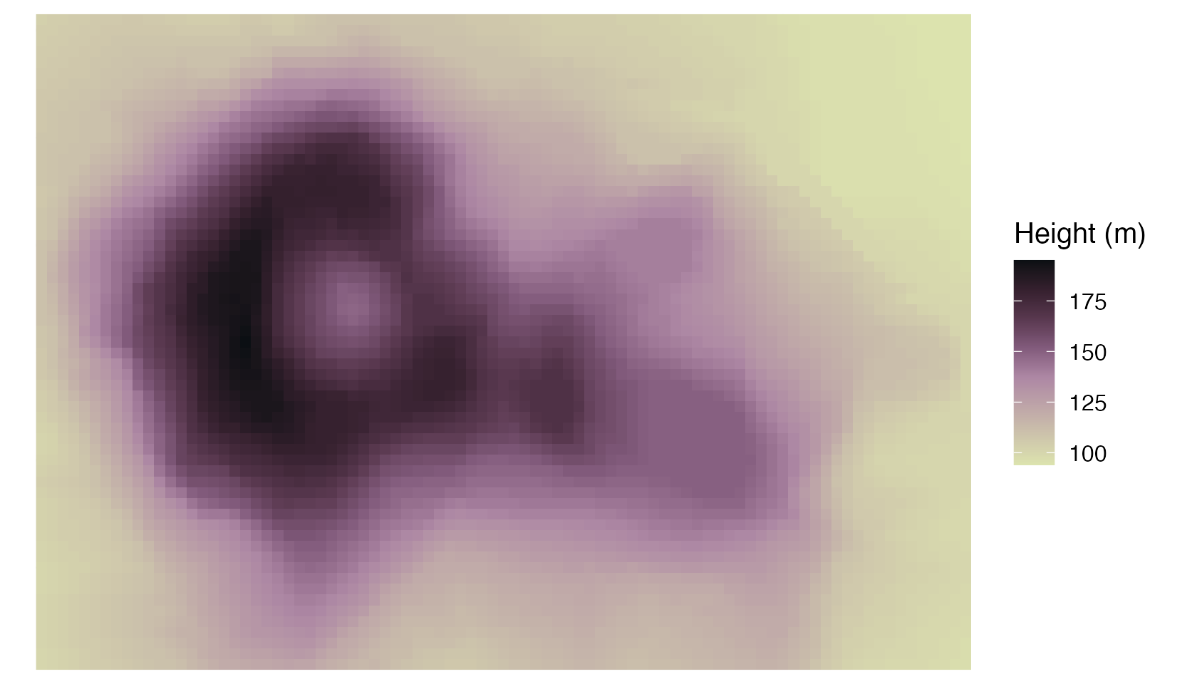
Diverging: values around a midpoint
Two dark arms meet in a light center, so the middle of the scale reads as neutral. Discrete subsets take both ends, then the center, then fill each arm evenly.
show_portinari(category = "diverging")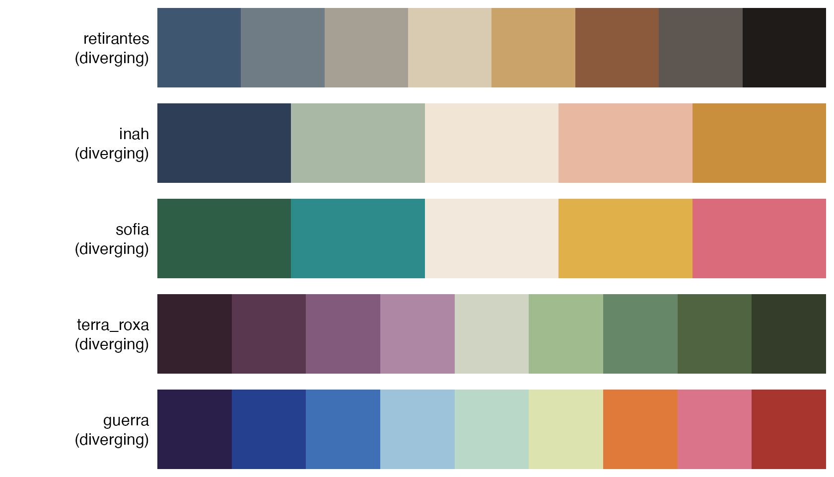
terra_roxa sets the plum of a coffee worker’s shirt
against the green of the plantation behind him, a classic purple-green
diverging scheme. It is colorblind-safe for all nine colors, which makes
it a good default for correlation matrices.
cors <- cor(mtcars)
cors_long <- data.frame(
  x = factor(rep(colnames(cors), each = ncol(cors)), levels = colnames(cors)),
  y = factor(rep(colnames(cors), times = ncol(cors)), levels = rev(colnames(cors))),
  r = as.vector(cors)
)
ggplot(cors_long, aes(x, y, fill = r)) +
  geom_tile(colour = "white", linewidth = 0.6) +
  geom_text(aes(label = sprintf("%.1f", r)), size = 2.8,
            colour = ifelse(cors_long$r < -0.3 | cors_long$r > 0.55, "white", "grey15")) +
  scale_fill_portinari("terra_roxa", type = "continuous", limits = c(-1, 1),
                       name = "Correlation") +
  coord_equal() +
  labs(x = NULL, y = NULL) +
  theme(panel.grid = element_blank())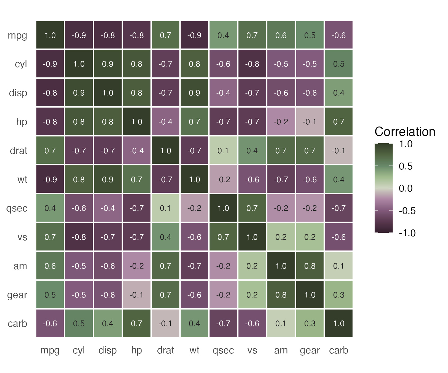
cars <- transform(mtcars, car = rownames(mtcars), diff = mpg - mean(mpg))
ggplot(cars, aes(diff, reorder(car, diff), fill = diff)) +
  geom_col() +
  scale_fill_portinari("guerra", type = "continuous", limits = c(-15, 15)) +
  labs(x = "mpg relative to the mean", y = NULL)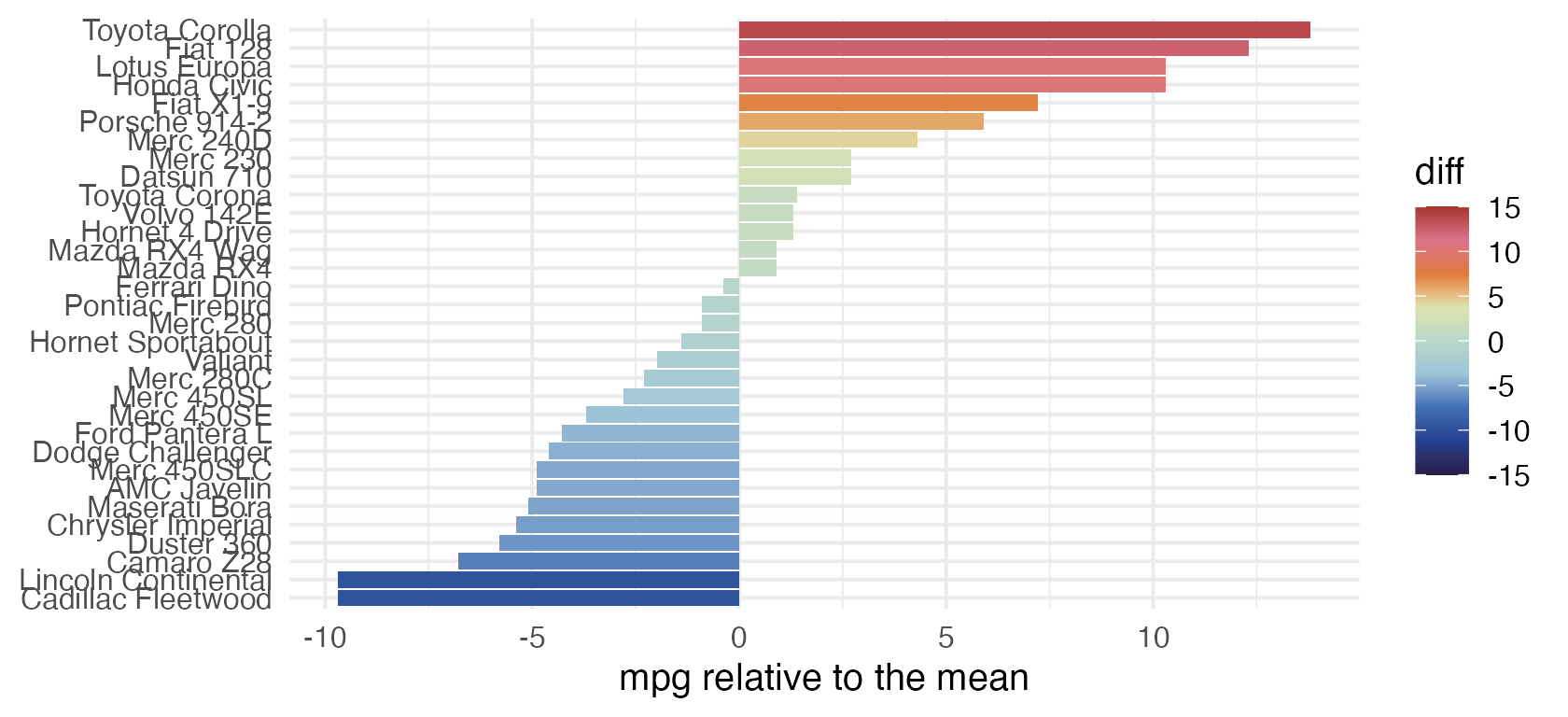
likert <- data.frame(
  question = rep(paste("Question", 1:4), each = 5),
  answer = factor(rep(c("Strongly disagree", "Disagree", "Neutral", "Agree", "Strongly agree"), 4),
                  levels = c("Strongly disagree", "Disagree", "Neutral", "Agree", "Strongly agree")),
  share = c(10, 20, 30, 25, 15, 5, 15, 20, 35, 25, 20, 25, 25, 20, 10, 8, 12, 30, 30, 20)
)
ggplot(likert, aes(share, question, fill = answer)) +
  geom_col() +
  scale_fill_portinari("retirantes", name = NULL) +
  labs(x = "%", y = NULL) +
  theme(legend.position = "bottom")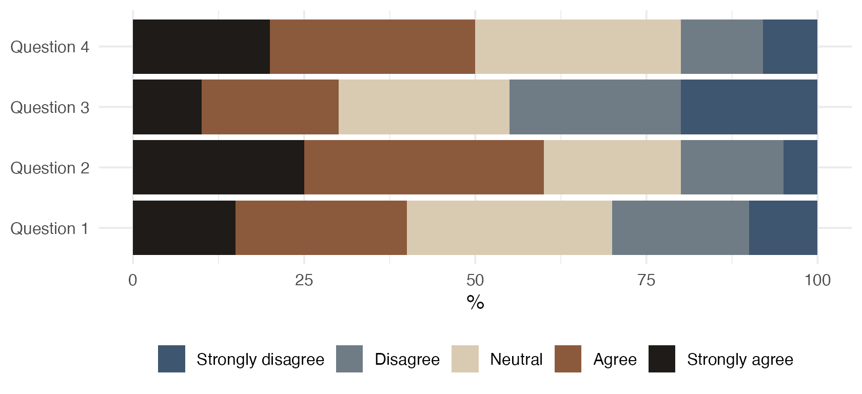
A Portinari canvas for your plots
theme_portinari() completes the look: a raw-linen
ground, firm drawn axis lines, earth-colored lettering and a painted
frame. The guerra and paz moods follow the two
United Nations panels.
ggplot(mtcars, aes(wt, mpg, colour = factor(cyl))) +
  geom_point(size = 3) +
  scale_color_portinari("paz", name = "Cylinders") +
  labs(title = "Fuel economy", subtitle = "Heavier cars travel less per gallon",
       x = "Weight (1000 lb)", y = "Miles per gallon") +
  theme_portinari()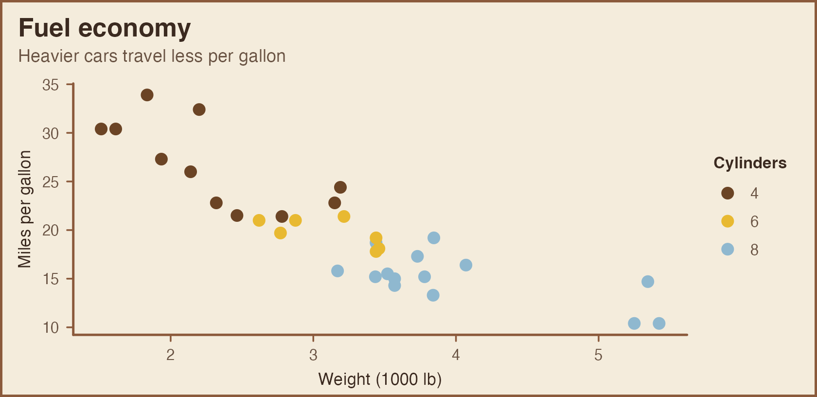
ggplot(faithfuld, aes(waiting, eruptions, fill = density)) +
  geom_raster() +
  scale_fill_portinari("guerra", type = "continuous") +
  coord_cartesian(expand = FALSE) +
  labs(title = "Old Faithful", subtitle = "The ground of War",
       x = "Waiting (min)", y = "Eruption (min)") +
  theme_portinari("guerra", grid = "none")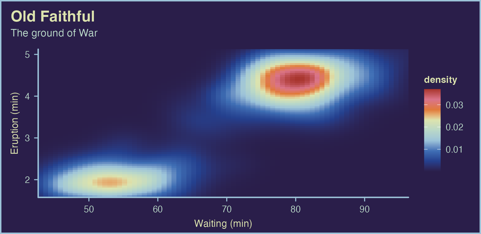
ggplot(mpg, aes(class, fill = drv)) +
  geom_bar(width = 0.75) +
  scale_fill_portinari("paz", name = "Drive") +
  labs(title = "Cars by class", subtitle = "The golden light of Peace",
       x = NULL, y = "Cars") +
  theme_portinari("paz")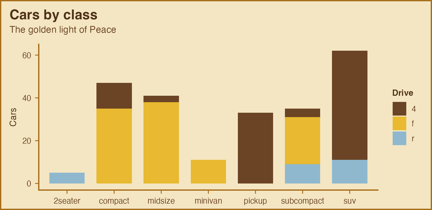
On a light mood, a palette’s lightest color sits close to the ground:
that suits filled areas, where it reads as neutral, but not points or
lines. On the guerra mood, prefer palettes other than
guerra and guerra_azul, whose darkest color is
the ground itself.
Colorblind safety
colorblind = TRUE restricts any palette to colors that
stay distinct under protanopia, deuteranopia and tritanopia
simulation.
portinari.pal("sofia", colorblind = TRUE)## <Portinari palette 'sofia'> 3 colors
## [1] "#2F5E46" "#F2E8DC" "#D96B7A"
portinari.cvd.check("sofia")## n normal protanopia deuteranopia tritanopia colorblind_safe
## 1 2 70.64010 18.331205 28.30175 82.36919 TRUE
## 2 3 55.02795 18.331205 28.30175 62.42223 TRUE
## 3 4 24.12647 7.530853 23.95855 21.86508 FALSE
## 4 5 24.12647 7.530853 23.95855 21.86508 FALSE